Introduction
Demand and supply determine the prices in market-driven economies. Everyone knows that, but many believe it is impossible to analyze demand and use that as a basis for automated pricing. Therefore, many companies implement rule based pricing on various metrics such as competitor prices, macroeconomic factors or available capacity. In this article, we present a case where a rule-based pricing solution is better than a static pricing, but also how demand-based pricing outperforms rule-based systems when it comes to results, adaptability and automation.
Case
In this fictional case, an events company organizes a small-town music festival. The event usually comes on sale five months in advance.
The traditional pricing for the event is a simple cost+ strategy, which takes the costs of organizing the event from the budget and adds a margin to the event. As a result, prices have stayed mostly the same over the years, with minor increases based on the increased expenses from labor and materials.
The sales have been consistent year over year, and the event usually sells the best a few weeks before the event. The sales consistently fill the venue, a local music hall. The venue has a capacity of 500.
A small-town country music festival:
- Time: June
- Prices: 40 USD for an adult ticket
- Attendance: 500 tickets sold
- Revenue: 40×500 = 20000 USD
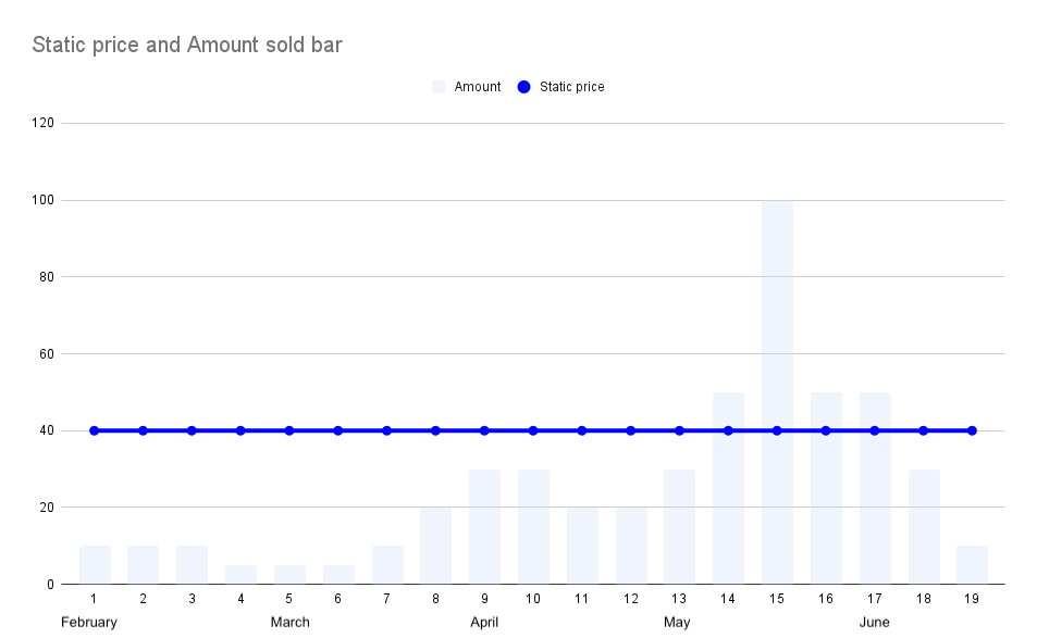
Figure 1: In the bar, chart you can see the sales volume per week and the static price represented by the line
A small-town country music festival:
- Revenue: 20000 USD
- Average price: 40 USD
- Volume: 500
This pricing model has worked well for the event-organizers in the past. However, they have been thinking about implementing a dynamic pricing solution to drive more sales early but limit the sales in case the event starts to fill up too quickly so that they do not need to sell out too cheaply.
Implementation of rules-based capacity pricing
The board of the company decided that initially the price should be set at a lower level and then increased in logical steps to sell the same amount but at a higher price. The first strategy they attempted was to tie the pricing to the capacity of the venue, to make the prices go up as the event fills up.
The event manager then estimated with their team what the correct steps should be. They came up with the following pricing strategy:
Capacity-based pricing strategy:
- First 100 tickets: 30 USD
- Tickets 100-200: 40 USD
- Tickets 200-300: 50 USD
- Tickets 300-400: 55 USD
- Tickets 400-500: 60 USD
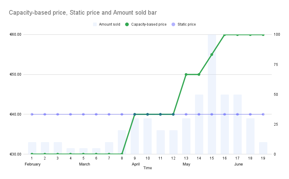
Figure 2: The green line represents the price movements over time for the capacity-based pricing compared to the static pricing
The sales went as expected, like in previous years, and the revenue significantly improved. The board was happy, and the customers did not seem to mind the price changes as they had been expecting price increases due to the previous rather stagnant pricing over the last few years.
Despite the lower price at the beginning of the year, people did not shift their behavior. The assumption is that they hardly make decisions about small festivals so long before. That resulted in the predictable sales pattern just before the festival again. As the sales stayed the same despite the price, the pricing model generated direct profit compared to the previous year.
Capacity-based pricing results:
- Revenue: 24,150.00 USD
- Average price: 41.84 USD
- Volume: 500
- The increase compared to static pricing: 20.75%
Implementation of rules-based time-bound pricing
The board was happy, but they wondered if they could raise the price even earlier before the peak sales to catch even more profit, as long as the volumes stay at similar levels. They decided to try a time-based pricing strategy because they believe they understand customer behavior from historical data. The event manager used data-driven estimates to choose the times to change the price. They came up with the following pricing strategy:
Time-based pricing strategy:
- February-March: 30 USD
- April: 45 USD
- May: 55 USD
- June: 60 USD
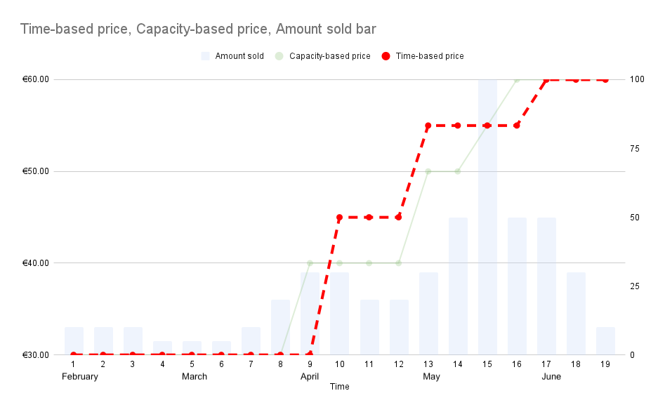
Figure 3: The red line represents the price movements over time for the time-based pricing compared to the capacity-based pricing in light green
Time-based pricing results:
- Revenue: 24,350.00 USD
- Average price: 42.37 USD
- Volume: 500
- The increase compared to static pricing: 21.75%
- The increase compared to capacity-based pricing: 0.8%
The board of directors was mildly disappointed with the results, as they had wished for a better increase in revenue compared to capacity-based pricing.
The benefits of this pricing strategy were that it was relatively easy to implement, and the hardest part was to decide what the steps should be and when to raise the prices.
Implementation of demand-driven dynamic pricing
Because of the previous year’s results, the board decided to apply more advanced dynamic pricing based on demand rather than the time before the event or the capacity of the venue.
The demand-based pricing uses sophisticated algorithms to estimate the demand for a given event and compares the actual demand over time to the estimated demand. If the demand is lower than expected, the algorithm lowers the price. Conversely, with high demand, the prices rise. This method helps the algorithm to price the event with smaller price movements and raise the price earlier than a more rigid rules-based pricing system would be able to. Similarly, the system would react quickly if sales are slower than expected and alert the event organizers early about the potential issue. The allowed price range is 30-60€, with a start price of 30€.
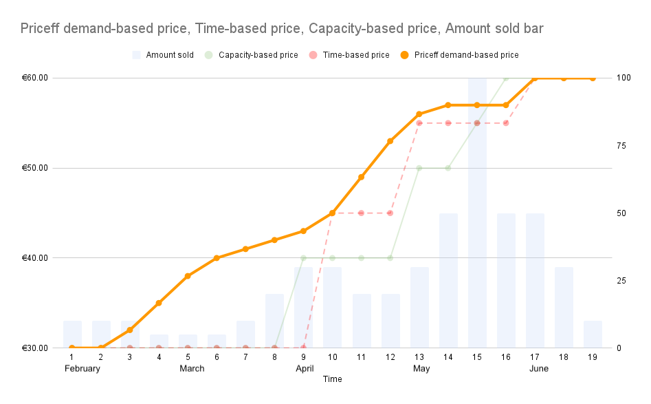
Figure 4: The orange line represents the Priceff demand-based price for the same sales volumes compared to the time (light red dashed) and capacity (light green) based pricing graphs
Demand-based pricing results:
- Revenue: 25,895.00 USD
- Average price: 46.58 USD
- Volume: 500
- The increase compared to static pricing: 29.48%
- The increase compared to capacity-based pricing: 7.23%
- The increase compared to time-based pricing: 6.34%
As you can see from the graph, instead of defining the times to raise the price, we raise the price earlier when the demand metric indicates that we have a new surge of demand which would sell out the event at that price. The demand curve is all about how steep the growth of cumulative sales is. Equally, demand-based dynamic pricing can be configured to lower the price if it looks like the event sells less well closer to the event. Events have a lot of fixed costs and upsell opportunities to customers, and it probably makes sense to fill up the venue even at a lower average ticket price. The expected demand is modeled by machine learning from historical sales, and the system reacts rapidly if the real-time demand varies up or down from the expected.
Conclusion
Demand can be estimated and those estimates can be used to build a dynamic pricing strategy that can adjust to demand fluctuations and find the optimal price for each moment automatically. All rule-based approaches are highly dependent on how well the rules and underlying data reflect customer behavior in-reality. Demand is the absolute measure of whether customers are willing to buy right now at the given price and all given other conditions, be them external or internal.
Demand-based dynamic pricing reacts quickly to changes in demand, naturally within given boundaries. Automated pricing is far more efficient than adjusting prices manually for a large number of products or services, especially if services are allocated to given timeslots, e.g. rentals, sports bookings, events.
In Figure 5, you can see the extra revenue comparing demand-based pricing and pricing that increases gradually either when capacity fills up or time passes. Note that this example is for an event that consistently sells out. For events that do not sell as well, the demand-based algorithm can also drive sales by lowering the price if the aim is to get volume and revenue at the expense of the price
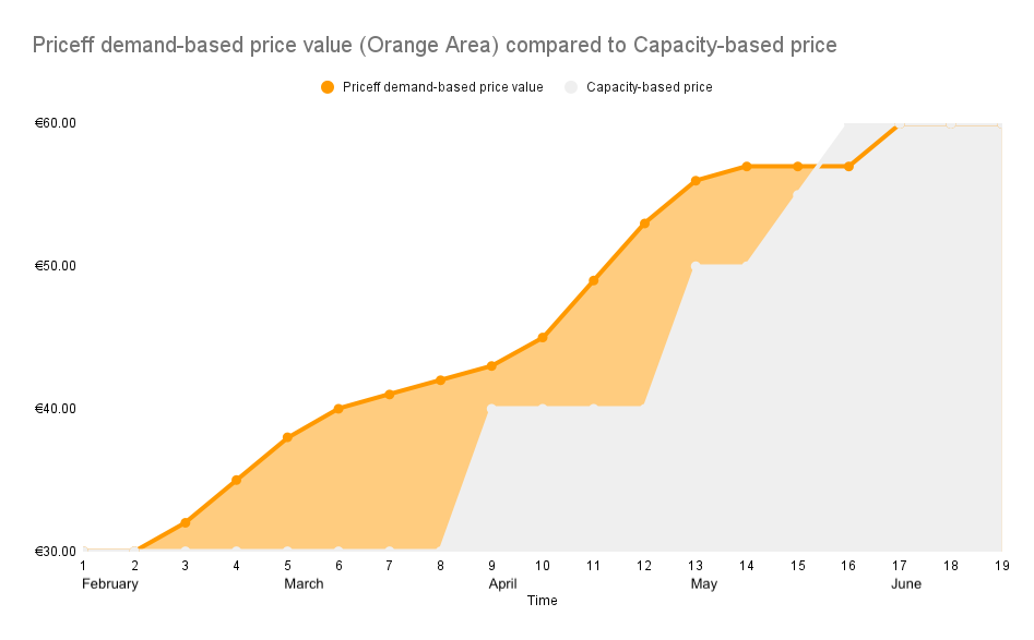
Figure 5: The orange area represents the potential gains of demand-based pricing compared to a simple capacity based pricing, in case of a successful event that sells well from early on.


